BinBayes.R
BinBayes.R is the software implementation for the paper "A Bayesian approach for the mixed effects analysis of repeated measures accuracy studies." which could be downloaded from here
Introduction
We assume that the user has both the R and JAGS software packages installed and is familiar with the basic structure and syntax of the R language. In addition, we also require the following three R packages: coda, lme4 and rjags. These packages can be installed from within R using the Package Installer from the main menu. To set up your system for using JAGS, do the following:
Download the current version of JAGS (4.2 as of 9/17/2016).
Install the current rjags package from CRAN. This can be done simply from within R using the Package Installer.
Once you have done that, a simple call to library('rjags') will be enough to run JAGS from inside of R.
The R function BinBayes.R requires five input variables as follows:
factor is a numeric indicator. 1 is for single-factor design and 2 is for two-factor design.
-
m_data is a matrix or data frame containing the data from your study.
- For single-factor design, this data frame should have four columns. The first column contains the subject identifier; the second column contains the item identifier; the third column contains the identifier for experimental condition; the fourth column holds a binary valued accuracy response. These columns should be in the following order: subject identifier, item identifier, identifier for experimental condition, accuracy response.
- For two-factor design, this data frame should have five columns. The first column contains the subject identifier; the second column contains the item identifier; the third column contains the identifier for factor 1; the fourth column contains the identifier for factor 2; the fifth column holds a binary valued accuracy response. These columns should be in the following order: subject identifier, item identifier, identifier for factor 1, identifier for factor 2, accuracy response.
link is a string that specifies the link function as ”Logit” or ”Probit”.
-
model_struct specifies the model structure.
For single-factor design, this is a number taking five possible values as follows:
- 1, baseline model with random subject and item effects with no effect of experimental condition.
- 2, model with random subject and item effects and with a fixed effect for the experimental condition.
- 3, model with random subject and item effects and where the effect of experimental condition varies across subjects.
- 4, model with random subject and item effects and where the effect of experimental condition varies across items.
- 5, model with random subject and item effects and where the effect of experimental condition varies across both subjects and items.
For two-factor design, this is a vector of three elements. The first two elements specify the model structure for factor 1 and factor 2 respectively. Each element can take values from 1 to 5 as with the specification of the single-factor design.The last element is either 0 or 1; if this value is 0 then no interaction between the two factors is included in the model while if this value is 1 an interaction is included in the model.
baseline is a string for single-factor design that specifies the label for the baseline condition. The software will automatically pick one condition as baseline if no specific condition is given. For two-factor design, this is a vector of two string variables that specifies the label of the bassline condition for factor 1 and factor 2 respectively.
As illustrated below, the output of the BinBayes.R function will consist of an object having five components with the following names:
- bic is the value of the BIC for the fitted model.
- waic is the value of the WAIC for the fitted model.
- post_summary is an mcmc list containing samples from the posterior distribution for all components of the fitted model.
- condition_level is the ordered condition level in the model. The first level would be the baseline if no specific condition is given as baseline condition.
- baseline is the baseline condition.
We will illustrate how to use BinBayes.R in the following three examples. Download BinBayes.R from here and save the directory to a known location on your hard drive.
Example 1 - Single-Factor Design
For this example, we were investigating the development of memory for visual scenes that occurs when one searches a scene for a particular object. We were specifically interested in what subjects might learn about other, non-target objects present in the scene while searching for the target object. In the first phase of the experiment, subject searched 80 scenes for a particular target object. In the test phase, they again searched the 80 scenes from the study phase as well as a set of 40 new scenes (new condition), looking for a specific target object in each case. For 40 of the scenes that had appeared in the first phase of the experiment, the target object was the same as in the first phase (studied condition), and for the other 40 scenes a new target was designated (alternate condition). In all 120 of these critical scenes, the target was present in the scene. Accuracy reflects whether or not the target was detected in the scene. Our primary interest was in whether there would be a benefit in the alternate condition, relative to the new condition, for having previously searched the scene (albeit for a different target). So the independent variable was scene type (studied, alternate, new) and the dependent variable was successful or failed detection of the target. There was also an additional set of scenes that did not contain the target that subjects were asked to search for, just to ensure that the task would be meaningful. Performance with these items was not analyzed. The dataset for this example can be downloaded here here and it has::
- 30 subjects
- 3 conditions
- 240 items
- 3550 total observations
- Overall accuracy 89.8%
To get started, let's download the BinBaye.R and save it in the same directory or folder with dataset Scenes3_Bayesian.txt.
# Path is the file directory where you save the BinBayes.R and dataset Prime3_Bayesian.txt should be in the same directory
 > path <- "/Users/Yin/Dropbox/BinBayes/BinBayes.R"

 # Load BinBayes.R
 > source(path)

 # Load required packages
 > library(coda)
 > library(lme4)
 > library(rjags)

# Read data into R
> accuracy <- read.table("/Users/Yin/Dropbox/BinBayes/Scenes3_Bayesian.txt", header=TRUE, na.strings='.',colClasses=c('factor','factor','factor','numeric'))
> #remove cases with missing values
> accuracy<-na.omit(accuracy)
> accuracy
     subj itemID cond Acc
1     s01   i001  std   1
2     s01   i004  alt   1
3     s01   i006  new   1
4     s01   i008  new   1
5     s01   i009  std   1
6     s01   i011  alt   1
7     s01   i014  new   1
8     s01   i016  new   1
9     s01   i017  std   1
10    s01   i020  std   1
11    s01   i022  std   0
12    s01   i024  std   1
13    s01   i026  new   1
14    s01   i027  new   1
15    s01   i029  std   1
16    s01   i032  std   1
17    s01   i034  alt   1
18    s01   i035  new   1
19    s01   i038  alt   1
20    s01   i039  std   1
21    s01   i042  std   1
.
.
.
.
Suppose we are interested in comparing model 1, which has no effect of the experimental condition and model 2, which has fixed effect for the experimental condition with logit link function, we can first compute BIC and WAIC for both models.
# Model 1 with Logit link
> L1_result <- BinBayes(1,accuracy, 1, "Logit")
Loading required package: Matrix
Linked to JAGS 3.4.0
Loaded modules: basemod,bugs
  |++++++++++++++++++++++++++++++++++++++++++++++++++| 100%
  |**************************************************| 100%
  |**************************************************| 100%
  |**************************************************| 100%

> L1_result$bic
[1] 2049.508
> L1_result$waic
[1] 1880.468
> L1_result$baseline
[1] std
Levels: alt new std
> L1_result$condition_level
[1] std alt new
Levels: alt new std


# Model 2 with Logit link
> L2_result <- BinBayes(1, accuracy, 2, "Logit")
> L2_result$bic
[1] 2020.746
> L2_result$waic
[1] 1835.745
> L2_result$baseline
[1] std
Levels: alt new std
> L2_result$condition_level
[1] std alt new
Levels: alt new std
According to the BIC and WAIC values, we can see that model 2 with random effects for subject and item and a fixed effect for condition is optimal among the these two models. Then we can get a posterior summary from model 2 by summary() function.
> summary(L2_result$post_summary)

Iterations = 12001:32000
Thinning interval = 1
Number of chains = 1
Sample size per chain = 20000

1. Posterior mean and standard deviation for each variable,
   plus standard error of the mean:

             Mean     SD  Naive SE Time-series SE
a[1]     -0.11448 0.9904 0.0070032       0.009571
a[2]     -0.85242 0.8024 0.0056739       0.007862
a[3]      0.10590 0.9522 0.0067328       0.009261
a[4]      0.09433 0.9397 0.0066448       0.008666
a[5]      1.05577 1.2407 0.0087731       0.011628
a[6]     -0.04343 0.9677 0.0068425       0.009498
a[7]      1.23382 1.1968 0.0084630       0.011032
a[8]      0.10627 0.9540 0.0067461       0.009359
a[9]      1.06573 1.2328 0.0087172       0.011379
a[10]    -2.55822 0.5976 0.0042253       0.007460
a[11]    -2.24377 0.6107 0.0043181       0.007147
a[12]    -0.14575 0.9604 0.0067909       0.009049
.
.
.

alpha[1]  0.00000 0.0000 0.0000000       0.000000  # Condition std
alpha[2] -0.90427 0.1715 0.0012128       0.003857  # Condition alt
alpha[3] -1.02556 0.1696 0.0011992       0.003634  # Condition new
.
.
.
b[27]    -0.30396 0.3240 0.0022910       0.004301
b[28]     0.76835 0.3971 0.0028078       0.004777
b[29]     0.35706 0.3825 0.0027050       0.004741
b[30]    -0.03684 0.3441 0.0024334       0.004709
beta0     3.84647 0.2384 0.0016859       0.009772
sigma_a   1.64579 0.1410 0.0009969       0.003578
sigma_b   0.70411 0.1253 0.0008858       0.001730
The notation for each of the model components is as follows:
| Model Component | Explanation |
|---|---|
| alpha[i] | Fixed Effect from Condition[i] |
| a[j] | Random Effect from Item[j] |
| b[k] | Random Effect from Subject[k] |
| beta0 | Model Intercept |
| sigma_a | Standard Deviation for Random Item Effect |
| sigma_b | Standard Deviation for Random Subject Effect |
Also, notice that the baseline condition is std for both models since we didn't specify the baseline condition at beginning. We can also set the baseline to new as follows:
> L2_new_result <- BinBayes(1,accuracy, 2, "Logit","new")
> L2_new_result$bic
[1] 2020.746
> L2_new_result$waic
[1] 1836.863
> L2_new_result$condition_level
[1] new alt std
Levels: alt new std
> L2_new_result$baseline
[1] "new"
Since the baseline condition is now new , the posterior summary for condition would also change as:
> summary(L2_new_result$poster_distribution)

Iterations = 12001:32000
Thinning interval = 1
Number of chains = 1
Sample size per chain = 20000

1. Posterior mean and standard deviation for each variable,
   plus standard error of the mean:

               Mean     SD  Naive SE Time-series SE
a[1]     -0.1381526 0.9597 0.0067864       0.009222
a[2]     -0.8483886 0.8117 0.0057399       0.008231
a[3]      0.1075865 0.9414 0.0066567       0.009286
a[4]      0.1155041 0.9463 0.0066913       0.009295
a[5]      1.0501409 1.2452 0.0088046       0.011279
a[6]     -0.0396419 0.9529 0.0067377       0.009271
a[7]      1.2152686 1.1842 0.0083734       0.011406
a[8]      0.1136061 0.9329 0.0065968       0.008816
a[9]      1.0356179 1.2262 0.0086704       0.011805
a[10]    -2.5505333 0.5896 0.0041692       0.007777
a[11]    -2.2260440 0.6115 0.0043236       0.007669
a[12]    -0.1168826 0.9798 0.0069280       0.009170
a[13]     1.2305091 1.2001 0.0084860       0.011587
a[14]     1.1816613 1.1963 0.0084591       0.011595
a[15]     1.0547813 1.2524 0.0088561       0.011643
a[16]     1.0478054 1.2214 0.0086366       0.011347
a[17]     1.1015207 1.2190 0.0086196       0.011925
a[18]    -1.9143807 0.6066 0.0042894       0.007095
a[19]     1.1166556 1.2123 0.0085726       0.011444
.
.
.
alpha[1]  0.0000000 0.0000 0.0000000       0.000000 # Condition new
alpha[2]  0.1209206 0.1464 0.0010351       0.002333 # Condition alt
alpha[3]  1.0376313 0.1717 0.0012139       0.002484 # Condition std
.
.
.
b[26]     0.5135574 0.3734 0.0026405       0.004417
b[27]    -0.2997185 0.3208 0.0022685       0.004270
b[28]     0.7657723 0.3889 0.0027497       0.004230
b[29]     0.3713921 0.3710 0.0026231       0.004368
b[30]    -0.0254439 0.3396 0.0024011       0.004399
beta0     2.7935181 0.2134 0.0015088       0.007985
sigma_a   1.6323807 0.1407 0.0009952       0.003600
sigma_b   0.7007261 0.1246 0.0008812       0.001655
Example 2 - Single-Factor Design
For this example, we were investigating the influence of a semantic context on the identification of printed words shown either under clear (high contrast) or degraded (low contrast) conditions. The semantic context consisted of a prime word presented in advance of the target item. On critical trials, the target item was a word and on other trials the target was a nonword. The task was to classify the target on each trial as a word or a nonword (this is called a "lexical decision" task). Our interest is confined to trials with word targets. The prime word was either semantically related or unrelated to the target word (e.g., granite-STONE vs. attack-FLOWER), and the target word was presented either in clear or degraded form. Combining these two factors produced four conditions (related-clear, unrelated-clear, related-degraded, unrelated-degraded). For the current analysis, accuracy of response was the dependent measure. The dataset for this example can be downloaded from here and it has:
- 72 subjects
- 4 conditions
- 120 items
- 8640 total observations
- Overall accuracy 95.4%
To get started, let's download the BinBaye.R and save it in the same directory or folder with dataset Prime3_Bayesian.txt.
 # Path is the file directory where you save the BinBayes.R and dataset Prime3_Bayesian.txt should be in the same directory
 > path <- "/Users/Yin/Dropbox/BinBayes/BinBayes.R"

 # Load BinBayes.R
 > source(path)

 # Read the data into R
 > accuracy <- read.table("/Users/Yin/Dropbox/BinBayes/Prime3_Bayesian.txt",header=TRUE, na.strings=’.’, colClasses=c(’factor’,’factor’,’factor’,’numeric’))
 > accuracy
     subj itemID cond Acc
1     S01   i001   UD   1
2     S01   i002   RD   1
3     S01   i003   UC   1
4     S01   i004   RD   1
5     S01   i005   RD   1
6     S01   i006   UC   1
7     S01   i007   RD   1
8     S01   i008   UD   1
9     S01   i009   RC   1
10    S01   i010   UD   1
.
.
.
Suppose we are interested in comparing model 1, model 2 and model 4 with Logit as the link function. We can compute the BIC and WAIC values as:
# Model 1 with Logit link
> L1_result <- BinBayes(1,accuracy,1,"Logit")
> L1_result$bic
[1] 2927.731
> L1_result$waic
[1] 2826.157

# Model 2 with Logit link
> L2_result <- BinBayes(1,accuracy,2,"Logit")
> L2_result$bic
[1] 2925.133
> L2_result$waic
[1] 2801.64


 # Model 4 with Logit link
> L4_result <- BinBayes(1,accuracy, 4, "Logit")
> L4_result$bic
[1] 2996.642
> L4_result$waic
[1] 2799.036
| Model | BIC | WAIC |
|---|---|---|
| Model 1 with Logit Link | 2927.731 | 2826.157 |
| Model 2 with Logit Link | 2925.133 | 2801.64 |
| Model 4 with Logit Link | 2996.642 | 2799.036 |
According to the BIC and WAIC values in the table above, we can see that model 4 has the lowest WAIC among these three models. We can then summarize the posterior distribution of L4 with the summary() function as:
> summary(L4_result$post_summary)

                    Mean      SD  Naive SE Time-series SE
a[1]           -1.666619 0.38431 0.0027175       0.005483
a[2]            1.039674 0.77228 0.0054608       0.007939
a[3]           -0.436582 0.52398 0.0037051       0.005583
a[4]            0.523383 0.67314 0.0047598       0.006237
a[5]            0.130259 0.61050 0.0043169       0.006002
a[6]            0.550793 0.68563 0.0048481       0.006804
a[7]            0.508255 0.67759 0.0047913       0.006294
a[8]           -0.462363 0.51865 0.0036674       0.005491
a[9]            0.523246 0.68582 0.0048495       0.006715
a[10]           1.032644 0.77398 0.0054729       0.007208
a[11]           1.052646 0.77478 0.0054785       0.007389
a[12]          -0.185695 0.56195 0.0039736       0.005674
a[13]           0.128977 0.62340 0.0044081       0.006219
.
.
alpha[1]        0.000000 0.00000 0.0000000       0.000000
alpha[2]        0.522522 0.15767 0.0011149       0.003081
alpha[3]        0.469008 0.15717 0.0011114       0.003916
alpha[4]        0.870208 0.17169 0.0012141       0.003330
.
.
.
b[72]           0.154551 0.33365 0.0023593       0.003061
beta0           3.220296 0.15636 0.0011056       0.004975
sigma_a         1.044492 0.10276 0.0007266       0.002024
sigma_alpha_a   0.307304 0.15130 0.0010699       0.024015
sigma_b         0.445203 0.08643 0.0006111       0.002314

2. Quantiles for each variable:

                   2.5%       25%        50%       75%    97.5%
a[1]           -2.40264 -1.927270 -1.677e+00 -1.416205 -0.88247
a[2]           -0.34187  0.503281  9.891e-01  1.529061  2.69899
a[3]           -1.39226 -0.803360 -4.587e-01 -0.096473  0.64460
a[4]           -0.68471  0.048638  4.834e-01  0.956490  1.93190
a[5]           -0.97531 -0.294504  9.742e-02  0.526003  1.39432
a[6]           -0.67287  0.080029  5.096e-01  0.978793  2.01615
a[7]           -0.71832  0.034044  4.702e-01  0.951443  1.92774
a[8]           -1.41925 -0.822585 -4.838e-01 -0.125123  0.63022
a[9]           -0.70916  0.044405  4.846e-01  0.964496  1.95642
a[10]          -0.34821  0.482410  9.873e-01  1.530585  2.67478
a[11]          -0.36522  0.518697  1.012e+00  1.544634  2.70457

.
.
.
b[72]          -0.46948 -0.069610  1.445e-01  0.364310  0.85110
beta0           2.92314  3.115602  3.216e+00  3.324324  3.53517
sigma_a         0.85986  0.973533  1.038e+00  1.109433  1.26308
sigma_alpha_a   0.08333  0.182168  2.862e-01  0.420978  0.61780
sigma_b         0.28170  0.386430  4.423e-01  0.501519  0.62269
The notation for each model component is as follows:
| Model Component | Explanation |
|---|---|
| alpha[i] | Fixed Effect from Condition[i] |
| a[j] | Random Effect from Item[j] |
| b[k] | Random Effect from Subject[k] |
| beta0 | Model Intercept |
| sigma_alpha_a | Standard Deviation for Random Effect between Condition and Item |
| sigma_b | Standard Deviation for Random Subject Effect |
| sigma_a | Standard Deviation for Random Item Effect |
To get the 95% HPD interval from the posterior distribution, we can use the HPDinterval() function as:
> HPDinterval(L4_result$post_summary)
[[1]]
                     lower        upper
a[1]           -2.41025325 -0.894806199
a[2]           -0.38651414  2.632236211
a[3]           -1.41609373  0.614345971
a[4]           -0.76273537  1.836882851
a[5]           -0.99880603  1.360993525
a[6]           -0.72229744  1.938909641
a[7]           -0.75741826  1.868160246
a[8]           -1.47657183  0.545669511
a[9]           -0.75937260  1.885694854
a[10]          -0.47287933  2.529157249
a[11]          -0.53205566  2.505668419
a[12]          -1.25500856  0.943159053
a[13]          -1.08890694  1.345130234
a[14]          -0.73722657  1.945710439
a[15]          -1.03913145  1.343106172

.
.
.
.
alpha[1]        0.00000000  0.000000000
alpha[2]        0.21653368  0.830800835
alpha[3]        0.16986439  0.784598683
alpha[4]        0.54651733  1.222875035
.
.
.
b[72]          -0.49810276  0.813090875
beta0           2.92129277  3.532019961
sigma_a         0.84947106  1.249148289
sigma_alpha_a   0.06478434  0.569423083
sigma_b         0.27834271  0.617972602
To create the density plots and boxplots summarizing the posterior distribution, in particular the condition effects, we can first use the varnames() function in R to see all the variable names in the post summary component of the fitted model. We then extract the corresponding variables to create posterior density plots and item effect boxplots for the parameters that we are interested in.
> varnames(L4_result$post_summary)
[1] "a[1]"         "a[2]"         "a[3]"         "a[4]"         "a[5]"
[6] "a[6]"         "a[7]"         "a[8]"         "a[9]"         "a[10]"
.
.
.
[671] "b[67]"      "b[68]"        "b[69]"        "b[70]"        "b[71]"
[676] "b[72]"      "beta0"        "sigma_a"      "sigma_alpha_a" "sigma_b"
To get the posterior density for "sigma_a", which is standard deviation for random item effect, we need to find the location of "sigma_a" in this mcmc list which is in column 678. Then we can get:
> plot(L4_result$post_summary[,678])

To create boxplots of condition effect by item, we can do as follows:
- Get the ordered condition level from condition_level.
- Reformat the post_summary part from result as a matrix by as.matirx() function.
- Use varnames() function to locate the columns of fixed effect of condition and mix effect between item and condition for the specific condition.
- Add the fixed condition effect to the corresponding mix effect columns.
- Use apply() function to find the median of columns obtained in (3) and sort them by order() function.
- Then use these ordered columns in (4) to create boxplot.
We select the second condition (RD) in the demonstration below:
> L4_result$baseline
[1] UD
Levels: RC RD UC UD

> L4_result$condition_level
[1] UD RD UC RC
Levels: RC RD UC UD

# Notice that RD is the second condition, we need to find the location of alpha[2] and all alpha_a[2,]s.
# By observing from varnames() result, we can see that alpha[2] is on the 122 column and all alpha_a[2,]s is located from 126 to 604 by every 4 columns.
# We have 120 items for each condition.

> index <- seq(from=126, to=604, by=4)

> rd_item <- as.matrix(L4_result$post_summary)[, index]

> colnames(rd_item) <- seq(from=1,to=120)

> # Fixed effect from second condition(RD)
> alpha_2 <- as.matrix(L4_result$post_summary)[,122]
> # Add the fixed effect to the mix effect

> for(i in  1:120){
+   rd_item[,i] <- rd_item[,i] + alpha_2
+ }
> # Sort the columns by median and get the index of sorted columns
> t2 <- apply(rd_item,2, median)
> order_index <- order(t2)

> # Swap the columns and their column names
> rd_item[,1:120] <- rd_item[,order_index]
> colnames(rd_item) <- order_index
> boxplot(rd_item,outline=FALSE,col="green")
> abline(h=0,col="red")
> title(main="RD effect by item")

Suppose we want to find out the label of the item that ranks 99th on the boxplot above and get the median of this item effect. We can do as follows:
# To get the label of item that ranks 99th in the boxplot above
> label_index_99th <- as.numeric(colnames(rd_item)[99])
> label_index_99th
[1] 20

# Item label in the dataset
> unique(accuracy$itemID)[label_index_99th]
[1] i020
120 Levels: i001 i002 i003 i004 i005 i006 i007 i008 i009 i010 i011 ... i120

# Find the posterior median and 95% HPD interval for this item effect
> median(rd_item[,99])
[1] 0.574344
> quantile(rd_item[,99], probs=c(0.025,0.975))
      2.5%      97.5%
-0.1418271  1.4581923
Also, a kernel density estimation for item identified above, which is the posterior distribution for the effect of experimental condition RD specific to item i020, could be plotted as:
# Posterior distribution for the effect of experimental condition RD specific to item i020.
p_99 <- density(rd_item[,99])
plot(p_99,main="Kernel Density Estimation for Item i020")

Example 3 - Two-Factor Design
The study produced trial-by-trial data for K = 73 subjects. Each subject experienced 480 trials in which a word prime was presented (requiring no response from the observer), followed by either a word or a nonword as a target that required a response. Subjects classified the targets as Word or Nonword. Our interest for the current analysis is in the accuracy (or error) rate for trials with Word targets, so trials with Nonword targets (240 trials per subject) are excluded. The word targets were words that occur with either high (HF) or low frequency (LF) in English (e.g., MORE vs TUSK). Word frequency is the first factor and the corresponding baseline condition in this case is LF. The second factor included in our analysis is viewing condition, whereby target items are presented either in Clear (full contrast) or Degraded (low contrast) displays, and we take the baseline condition for this factor to be the Degraded condition. That is:
- 73 subjects.
- 2 conditions for first factor.
- 2 conditions for second factor.
- 240 items.
- Total number of observations is 17,520.
- Overall accuracy 95.2%
Example dataset could be downloaed from here.
#read in dataset two factor dataset
accuracy <- read.table("/Users/Yin/Dropbox/data_set/Prime1A raw collated.txt", header=TRUE, na.strings='.',colClasses=c('factor','factor','numeric','factor','factor','factor','factor','factor','numeric','factor'))

#only keep the columns that are required for this analysis
keep<-c('S', 'TargetShown','Contrast', 'TargetType', 'score')
accuracy<-accuracy[,keep]

#remove trials where TargetType=NW
accuracy<-accuracy[accuracy$TargetType!='NW',]
accuracy<-droplevels(accuracy) #make sure NW is dropped as an unused factor level

#remove cases with missing values
accuracy<-na.omit(accuracy)

#convert the response to 0/1
accuracy$score<-as.numeric(accuracy$score=='C')

#
P22_0 <- BinBayes(factor = 2, m_data = accuracy, model_struct=c(2, 2, 0), link = "Probit")
  |++++++++++++++++++++++++++++++++++++++++++++++++++| 100%
  |**************************************************| 100%
  |**************************************************| 100%
  |**************************************************| 100%

# BIC
> P22_0$bic
[1] 5662.337

# WAIC
> P22_0$waic
[1] 5486.221

# Baseline condition for factor 1 and factor 2
> P22_0$baseline
[[1]]
[1] Degraded
Levels: Clear Degraded

[[2]]
[1] LF
Levels: HF LF
| Model | Link | Model Structure for Factors | WAIC | BIC |
|---|---|---|---|---|
| LM0N0I0 | Logit | Null | 5515 | 5673 |
| LM2N1I0 | Logit | F1 - fixed, F2 - null | 5500 | 5666 |
| LM2N2I1 | Logit | F1*F2 - fixed | 5498 | 5664 |
| LM3N2I0 | Logit | F1*Subject, F2- fixed | 5499 | 5683 |
| LM4N2I0 | Logit | F1*Item, F2- fixed | 5500 | 5682 |
| PM2N2I0 | Probit | (F1 + F2) - fixed | 5486 | 5662 |
To get the 95% HPD interval from the posterior distribution, we can use the HPDinterval() function as:
> HPDinterval(P2_0$post_summary)
[[1]]
                lower        upper
a[1]     -0.219135797  0.749688114
a[2]     -0.341859685  0.639471948
a[3]     -0.720883002  0.076366054
a[4]     -0.334839962  0.640257030
a[5]     -0.306967616  0.688504212
a[6]     -0.339510833  0.659315384
a[7]     -0.627972208  0.211136797
a[8]     -1.252435170 -0.627273741
a[9]     -0.570881030  0.212873340
a[10]    -0.212541085  0.853847137
a[11]    -0.232267882  0.711368142
a[12]    -0.703102888  0.032425345
a[13]    -0.408160671  0.522426867
a[14]    -1.309048728 -0.695067831
a[15]    -0.226041495  0.717749790
a[16]    -0.532365131  0.330189850
a[17]    -0.106462096  0.919521026
.
.
.
.
.
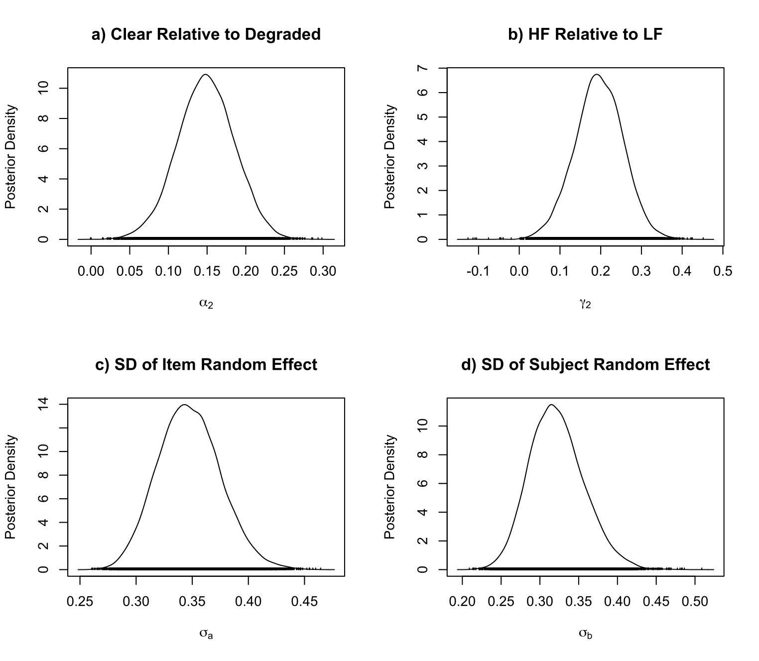
For the preferred model P220, we can plot the posterior density for the effect of clear contrast realtive to degraded contrast, and other posterior densities as follow:
# Using and varnames() function to locate the correspoding columns.
> varnames(P22_0$post_summary)
  [1] "a[1]"     "a[2]"     "a[3]"     "a[4]"     "a[5]"     "a[6]"
  [7] "a[7]"     "a[8]"     "a[9]"     "a[10]"    "a[11]"    "a[12]"
 [13] "a[13]"    "a[14]"    "a[15]"    "a[16]"    "a[17]"    "a[18]"
 [19] "a[19]"    "a[20]"    "a[21]"    "a[22]"    "a[23]"    "a[24]"
.
.
.
.
241] "alpha[1]" "alpha[2]" "b[1]"     "b[2]"     "b[3]"     "b[4]"
[247] "b[5]"     "b[6]"     "b[7]"     "b[8]"     "b[9]"     "b[10]"
[253] "b[11]"    "b[12]"    "b[13]"    "b[14]"    "b[15]"    "b[16]"
[259] "b[17]"    "b[18]"    "b[19]"    "b[20]"    "b[21]"    "b[22]"
[265] "b[23]"    "b[24]"    "b[25]"    "b[26]"    "b[27]"    "b[28]"
[271] "b[29]"    "b[30]"    "b[31]"    "b[32]"    "b[33]"    "b[34]"
[277] "b[35]"    "b[36]"    "b[37]"    "b[38]"    "b[39]"    "b[40]"
[283] "b[41]"    "b[42]"    "b[43]"    "b[44]"    "b[45]"    "b[46]"
[289] "b[47]"    "b[48]"    "b[49]"    "b[50]"    "b[51]"    "b[52]"
[295] "b[53]"    "b[54]"    "b[55]"    "b[56]"    "b[57]"    "b[58]"
[301] "b[59]"    "b[60]"    "b[61]"    "b[62]"    "b[63]"    "b[64]"
[307] "b[65]"    "b[66]"    "b[67]"    "b[68]"    "b[69]"    "b[70]"
[313] "b[71]"    "b[72]"    "b[73]"    "beta0"    "gamma[1]" "gamma[2]"
[319] "sigma_a"  "sigma_b"

# Using the densplot() from coda package to plot the posterior density

> library(coda)
> par(mfrow=c(2, 2))
> densplot(P22_0$post_summary[,242], xlab = expression(alpha[2]), ylab="Posterior Density")
> title(main="a) Clear Relative to Degraded")
> densplot(P22_0$post_summary[,318], xlab = expression(gamma[2]), ylab="Posterior Density")
> title(main="b) HF Relative to LF")
> densplot(P22_0$post_summary[,319], xlab = expression(sigma[a]), ylab="Posterior Density")
> title(main="c) SD of Item Random Effect")
> densplot(P22_0$post_summary[,320], xlab = expression(sigma[b]), ylab="Posterior Density")
> title(main="d) SD of Subject Random Effect")